This is a summary of doing human action recognition using Fisher Vector with (Improved) Dense Trjectory Features(DTF) and STIP features on UCF 101 dataset(http://crcv.ucf.edu/data/UCF101.php). In the STIP features, two low-level visual features HOG and HOF are integrated, with dimensions 72 and 90 respectively. The (improved) DTF employ more features(TR, HOG, HOF and MBHx/MBHy) with longer dimensions.
You can find my Matlab code from my GitHub Channel:
Dense Trajectory Features
For some details of DTF, please refer to my previous DTF notes.
Pipeline
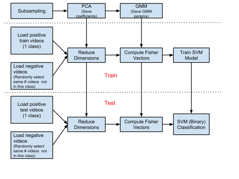
The pipeline of integrating DTF/STIP features and Fisher vectors is shown in Figure 1. The first step is subsampling a fixed number of STIP/DTF features(in my implementation, 1000) from each video clip in training list, which will be used to do PCA and train Gaussian Mixture Models(GMMs).
After getting the PCA coefficients and GMM parameters, treat UCF 101 video clips action by action. For each action, first load all train videos in this action(positive videos), and then randomly load the same number of video clips not in this action(negative videos). All of the loaded videos are multiplied with the saved PCA coefficients in order to reduce dimensions and rotate matrices. Fisher vectors are computed for each loaded video clip. Finally a binary SVM model is trained with both the positive and negative Fisher vectors.
When dealing with the test videos, similar process is adopted. The only difference is that the Fisher vectors are used for SVM classification, which is based on the SVM model trained with training videos.
 .
.
To well utilize the STIP or DTF features, features(HOG, HOF, MBH, etc.) are treated separately and they are only combined(simple concatenation) after computing Fisher vectors before linear SVM classification.
Pre-processing
STIP Features
The offcial STIP features are stored in class, which means that all the STIP info of all video clips in each class are mixed together in a file. To extract STIP features for each video, I wrote a script mk_stip_data to separate STIP features for each video clip. And all the following operations are based on each video clip.
DTF Features
Since the DTF features are “dense”(which means a lot of data), it took me 4~5 days to exact the (improved) DTF features of UCF 101 clips with the dedault parameters on a modern Linux desktop(I used 10 threads for extraction in paralle). The installation of DTF tools was also a very tricky task.
To save space, all the DTF features were compressed using script gzip_dtf_files. For UCF101, it would cost about 500GB after compression. And the required space would be doubled if no compression. If you don’t want to save the DTF features, you can call the DTF tools in Matlab and discard the extracted features.
Fisher Vector
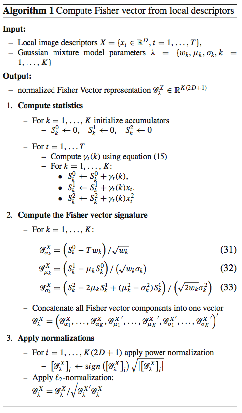
The Fisher Vector (FV) representation of visual features is an extension of the popular bag-of-visual words (BOV)[1]. Both of them are based on an intermediate representation, the visual vocabulary built in the low level feature space. A probability density function (in most cases a Gaussian Mixture Model) is used to model the visual vocabulary, and we can compute the gradient of the log likelihood with respect to the parameters of the model to represent an image or video. The Fisher Vector is the concatenation of these partial derivatives and describes in which direction the parameters of the model should be modified to best fit the data. This representation has the advantage to give similar or even better classification performance than BOV obtained with supervised visual vocabularies.
Following is the algorithm of computing Fisher vectors from features(actually I implemented this algorithm in Matlab, and if you are interested, please refer here):
 .
.
During the subsampling of STIP features, I randomly chose 1000 HOG or HOF features from each training video clip. For some videos, if the total number of features were less than 1000, I would use all of their features. All the subsampled features are square rooted after L1 normalization.
After that, the dimensions of the subsampled features were reduced to half of their original dimensions by doing PCA. At this step, the coefficients of PCA were recorded, which would be used in later. The GMMs were trained with the half-sized features, and the parameters of GMMs(i.e. weight, mean and covariance) were stored for the following process. In my program, the GMM code implemented by Oxford Visual Geometry Group(VGG) is used, which eventually call VLFeat. In my code, 256 Gaussians were used.
When computing the Gaussians, sometimes value Inf will be returned. For the Inf entries, a very large number(in my code, 1e30) is assigned instead to make the subsequent computation smoother. Before the L2 and power normalization, the unexpected NaN entries are replaced by a large number(in my implementation, 123456).
SVM Classification
Binary SVM classification(LIBSVM) is used in my implementation. For each action, positive video clips are labeled as 1 while negative videos are as labeled -1 during training and test. In my code, SVM cost is set to 100. The option of SVM training is:
-t 0 -s 0 -q -c 100 -b 1.
Results
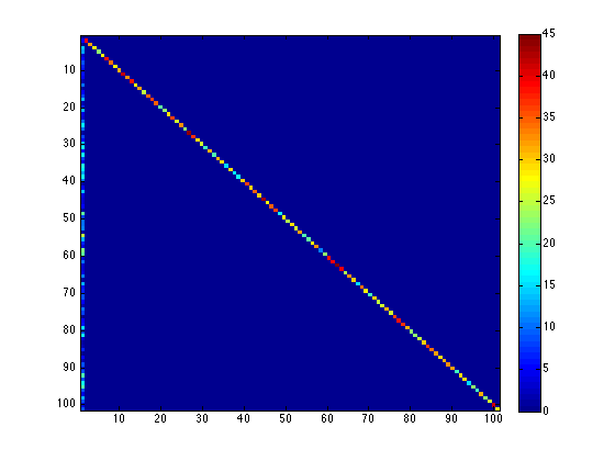
The action recognition accuracy of all the 101 actions was 77.95% when using above pipeline and STIP features. And the confusion matrix is shown in Figure 3.
The mean accurary of the fist 10 actions with DTF features was 90.6%, while the STIP was only 84.32%. The mean accuracy of the whole UCF 101 data(train/test list 1) was around 85% using DTF features, about 8% higher than using BOV representations(internal test). And the best result I got with the ISA neural network on UCF 101 was only 58% in November, 2013.
Conclusion
It is obvious that Fisher vector can lead to better results than Bag-of-visual words in action recognition. Compared to other low-level visual features, DTF features have more advantages in action recognition. However, in the long run I still believe deep learning methods - when deep neural networks could be trained with millions of vidios[5], they would learn more info from scratch and achieve state-of-the-art accuracy.
References
- Gabriela Csurka, Florent Perronnin, Fisher Vectors: Beyond Bag-of-Visual-Words Image Representations , Communications in Computer and Information Science Volume 229, 2011, pp 28-42.
- Chih-Chung Chang and Chih-Jen Lin. Libsvm: A library for support vector machines. ACM Trans. Intell. Syst. Technol., 2(3):27:1–27:27, May 2011.
- Heng Wang and Cordelia Schmid. Action Recognition with Improved Trajectories. In ICCV 2013 - IEEE International Conference on Computer Vision, Sydney, Australia, December 2013. IEEE.
- Jorge Sanchez, Florent Perronnin, Thomas Mensink, and Jakob Verbeek. Image Classification with the Fisher Vector: Theory and Practice. International Journal of Computer Vision, 105(3):222–245, December 2013.
- Andrej Karpathy, George Toderici, Sanketh Shetty, Thomas Leung, Rahul Sukthankar, and Li Fei-Fei. Large-scale video classification with convolutional neural networks. In CVPR, 2014.