Just like many people, I also own a very limited number of stocks. Although I tried my best to massage my portfolio(based on my guess, feeling and luck) last year, its year-end return was only about 3.5%. Compared to the S&P500’s 12% return, the poor performance shocked me. So I decided to study some formal computational stock analysis techniques. This post is the summary of what I learnt and developed. For the complete code, please refer to stock_analysis in my Github.
All of the methods/strategies mentioned in this post are collected from Internet or books, so there’s no guarantee for the correctness and validness.
Data Preparation
For personal use, the most popular language for stock analysis is Python, and the most convenient library is Pandas, which mainly depends on Numpy. So all the following discussions are based on Python Pandas.
To analyze stocks, we need a lot of data, like the history quotes, stock statistics, financial analysis, and etc. For my personal use, only free data sources are involved.
History Quotes
The history stock quotes can be downloaded using pandas_datareader, which was part of the Pandas before but now an independent library. The pandas_datareader.data.DataReader() could download the history quotes for one or a list of stock ticker(s). When passing one stock ticker, the DataReader() returns quotes as a Pandas DataFrame (2-D). When using a list of tickers as parameter, DataReader() returns Pandas Panel (3-D).
Following is a simple example of how it works:
import pandas as pd
import datetime as dt
import pandas_datareader.data as web

start_date = pd.to_datetime('2016-01-01').date()
end_date = dt.datetime.today().date()
quotes = web.DataReader('AAPL', 'yahoo', start_date, end_date)
Then the quotes should contain the DataFrame of Apple’s history quotes:
In [27]: print(quotes.iloc[:10,].to_string())
                  Open        High         Low       Close    Volume   Adj Close
Date
2016-01-04  102.610001  105.370003  102.000000  105.349998  67649400  102.612183
2016-01-05  105.750000  105.849998  102.410004  102.709999  55791000  100.040792
2016-01-06  100.559998  102.370003   99.870003  100.699997  68457400   98.083025
2016-01-07   98.680000  100.129997   96.430000   96.449997  81094400   93.943473
2016-01-08   98.550003   99.110001   96.760002   96.959999  70798000   94.440222
2016-01-11   98.970001   99.059998   97.339996   98.529999  49739400   95.969420
2016-01-12  100.550003  100.690002   98.839996   99.959999  49154200   97.362258
2016-01-13  100.320000  101.190002   97.300003   97.389999  62439600   94.859047
2016-01-14   97.959999  100.480003   95.739998   99.519997  63170100   96.933690
2016-01-15   96.199997   97.709999   95.360001   97.129997  79010000   94.605802
Note that since the market closed on 01/01/2016, the start date is automatically rounded to the first business day followed.
Stock Statistics
The stock statistics from Yahoo Finance are also very useful. Basically there are two options to download them - parsing from Yahoo Finance URL or querying using Yahoo Query Language(YQL). For the former case, webpage Downloading Yahoo data explains the URL format and tags. And herval/yahoo-finance lists more tags. For the YQL case, lukaszbanasiak/yahoo-finance integrates it into a library.
Examples of downloading stats via URL and YQL can be found from functions get_symbol_yahoo_stats_url and get_symbol_yahoo_stats_yql in my stock analysis library.
Financial Analysis
My current implmentation downloads financial statements from Google Finance using selenium. The selenium webdriver will bring up a browser(e.g. Chrome, Firefox, etc.) window and open the Google Financials page. I wrote a function parse_google_financial_table to parse the financial tables.
However, there are too many drawbacks to the current selenium + Google Finance solution, because (1) selenium needs start web browser, which is pretty slow; (2) Google Finance only provides statements for the past 4-5 quarters or 4 years; and (3) many raw fiancial data are not available in Google Finance…
A more promising candidate is pystock-crawler, which can directly parse and download 10-Q and 10-K filings from SEC EDGAR. Unfortunately, pystock-crawler still doesn’t support Python 3.x, and I don’t want to switch to Python 2.7. So I haven’t tried it by myself.
In addition to the aforementioned data, the insider trading and trading events are also very helpful. But I haven’t got chance to try them.
Data Processing
As stock-related data can be analyzed from many different aspects, a lot of indicators/features have been invented. My superficial understanding is that, technical analysis focuses on history quotes, while fundamental analysis pays more attention to the financial statements. Actually the stats data downloaded from Yahoo Finance and the financial data from Google Finance are already processed data by experts. So this part only covers the commonly used indicators of stock quotes.
Return On Investiment(ROI)
ROI is also called Rate Of Return, which measures the gain/loss of your stock investment in a given period. It’s defined as:
Total Stock Return = ((P1 - P0) + D) / P0
where
	P0 = Initial Stock Price
    P1 = Ending Stock Price
    D  = Dividends
Source code: return_on_investment
Moving Average
Moving average is widely used for smoothing stock data. The Simple Moving Average(SMA) calculates the mean prive of the previous n days. And the Exponential Moving Average(EMA) gives more credits to the most recent quote. In my implementation, the following algorithm is used to calculate EMA:
n: time periods in days
SMA := mean(n-day quotes)
multiplier := (2 / (n + 1))
EMA := (ClosePrice - EMA(previous day)) * multiplier + EMA(previous day).
The corresponding Python code is:
def moving_average(x, n=10, type='simple'):
    x = np.asarray(x)
    if type == 'simple':
        # SMA
        w = np.ones(n)
        w /= w.sum() # weights
        avg = np.convolve(x, w, mode='full')[:len(x)]
        avg[:n] = avg[n]
    else:
        # EMA
        avg = np.zeros_like(x)
        avg[:n] = x[:n].mean() # initialization
        m = 2/(n+1) # multiplier
        for i in np.arange(n,len(x)):
            avg[i] = (x[i] - avg[i-1]) * m + avg[i-1]
    return avg
Moving Average Convergence/Divergence(MACD)
The MACD series is the difference between a “fast” (short period) exponential moving average (EMA), and a “slow” (longer period) EMA of the price series. The average series is an EMA of the MACD series itself. The MACD indicator (or “oscillator”) is a collection of three time series calculated from historical price data: the MACD series proper, the “signal” or “average” series, and the “divergence” series which is the difference between the two.
The most commonly used days for MACD are 12, 26, and 9, that is, MACD(12,26,9), which means that
MACD Line = (12-period EMA – 26-period EMA)
Signal Line = 9-period EMA
Histogram = MACD Line – Signal Line
Source code: macd
Momentum
Momentum measures the rate of the trending(rise or fall) in stock prices. It’s defined as
Momentum = (Today's closing price) - (Closing price n days ago)
A similiar trending indicator is Rate of Change(ROC), which is defined as
ROC = ((current value) / (previous value) - 1) * 100
Relative Strength Index(RSI)
RSI is an oscillator to identify the trend, which ranges from 0 to 100, with a value greater than 70 indicating an overbought condition and a value lower than 30 indicating an oversold condition. And a RSI greater than 50 can indicate an uptrend and a RSI less than 50 indicates a downtrend.
The standard algorithm of calculating RSI is:
              100
RSI = 100 - --------
             1 + RS
RS = Average Gain / Average Loss

The very first calculations for average gain and average loss are simple 14 period averages.

First Average Gain = Sum of Gains over the past 14 periods / 14.
First Average Loss = Sum of Losses over the past 14 periods / 14.

The second, and subsequent, calculations are based on the prior averages and the current gain loss:

Average Gain = [(previous Average Gain) x 13 + current Gain] / 14.
Average Loss = [(previous Average Loss) x 13 + current Loss] / 14.
Source code: rsi
Stochastic Oscillator (%K)
The stochastic oscillator, represented by the symbol %K, is based on a window period that typically spans 14 trading days, where the highest high and the lowest low are selected from the range, and the last closing price are used to calculate %K. %K = 0 when the last close is also the low for the window period.
The stochastic oscillator can be calculated by:
Stochastic Oscillator(%K) = (Close Price - Lowest Low) / (Highest High - Lowest Low) * 100
Fast %D = 3-day SMA of %K
Slow %D = 3-day SMA of fast %D
Source code: stochastic
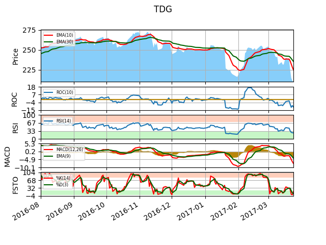
All of these indicators can be plotted into one graph:
from stock_analysis import Symbol

tdg = Symbol('TDG')
tdg.plot()
Strategies
As a newbie, I don’t know many stock trading strategies. Most of my time were spent on finding good and cheap stocks. So I sitll don’t know anything about stock prediction.
The most practicle strategy suitable(I believe) for personal stock trading that I have found, is the Magic Formula Investing from The Little Book That Beats the Market. I also implemented this strategy in my stock analysis library. My version doesn’t strictly follow Greenblatt’s strategy, because I still cannot find all the needed data. But I believe it already has the core of this strategy.
Example of how to use this strategy:
from stock_analysis import *
sp500 = SP500()   # define an index
sp500.get_financials() # download financial data Google Finance, a bit slow
sp500.get_stats() # calculate key statistic features
sp500_value = value_analysis(sp500)  # do the value analysis
Summary
I want to restate what Greenblatt explained in The Little Book That Beats the Market here:
Stock prices move around wildly over very short periods of time, but this does not mean that the values of the underlying companies have changed very much during that same period.
So always buy shares of a company only when they trade at a large discount to TRUE VALUE as investing with a margin of the safety.
Companies that achieve a high return on capital are likely to have a special advantage of some kind. That special advantage keeps competitors from destroying the ability to earn above-average profits.
But I also agree another point that Greenblatt discussed:
Puting all the time and effort into stock market investing isn’t a very productive use of time.
More than 95% of the stock trading back and forth each day is probably unnecessary.
Do not waste too much of the future potential. There are higher and better uses of your time and intellect.